explore machine learning applications for fisheries management
The project goal was to build a machine learning algorithm to automatically detect and classify 5 pre-selected species from existing videos at a desired accuracy (99%). We analyzed the prediction results and made recommendations for future applications.
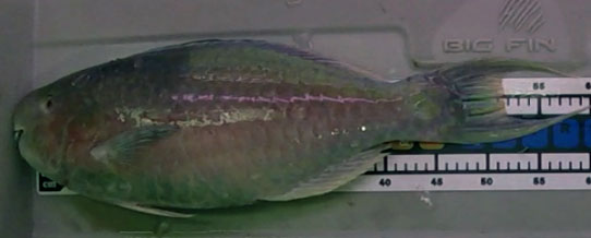
Video 1. Clip from bio-sampling video (forwarded X4)
Table 1. 5 species were selected to be used for the classification project.
Species
Name
Scarus rubroviolaceus
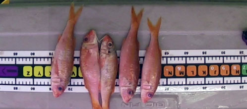
Lutjanus kasmira
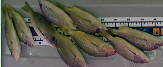
Mulloidichthys vanicolensis
Acanthurus triostegus
Acanthurus olivaceus
Data
In order to use machine learning to solve our task, we need to have annotated data created from the raw video files. We must label the fish in an image with its correct species and a draw bounding box around that fish. We restrict our interest
to the fish being measured by the technician; this allows us to have at most one label per image at a time and thus formulate the problem as a localization task.
Clay Sciences annotation software was selected as the annotation tool for this project. Videos are uploaded and associated metadata (classification and identification information) are
entered in advance. As videos are played, annotators manually draw bounding boxes around the fish. At the end of each video, annotated data can be downloaded in json data format. In total, these 18 videos were a cumulative of 195 minutes in
length, broken down into 349,491 frames (139,813 frames with fish). The bio-sampling videos have different length ranging from 5 to 15 minutes.
Machine Learning Project Structure
Data Collection
Data are collected to be used to train and validate the classification neural network. We are using data that were collected for other purposes (bio-sampling project). There was no additional data collected for this project.
Data Annotation
Data annotation is the task of labelling data (video). We annotate the video to create the "ground truth": where the fish is (detection) and what it is (classification). During the data annotation, we manually draw a box around a fish and label what it
is.
Data Augmentation
Data augmentation is a technique to increase the diversity of available by making modifications to the existing data. Images taken in the field may vary in zoom levels, lighting intensity, blurriness, size, etc. We apply data preprocessing to put the
data into a standard form and data augmentation to make our models perform well in varying conditions.
Build Neural Network
Artificial Neural Network algorithm is used to build the detection and classification. We build the neural network that will use the data and accuractely detect and classify the species.
Train the data and Validate
Spliting the data into training and testing, we train the neural network and validate the results using various evaluation matrix. The process is repeated with some tuning of parameters until a desired accuracy is obtained (if possible)
Methods
Data Augmentation
Images taken in the field (or video files) may vary in zoom levels, lighting intensity, blurriness, size, etc. Therefore, we apply data pre-processing to standardize the data and use augmentation techniques to ensure our models perform well in varying
conditions.
We use the following techniques:
Resizing and cropping: The standard input size to neural networks is 224 pixels by 224 pixels. If the images are not at this size, then we resize the smaller dimension to be 224 and take a random crop from the resulting rectangular image. The resizing
is done once as a form of preprocessing and the cropping is performed on the fly to make the model robust to different camera locations.
Horizontal flips, translations, rotations, projections, zoom-level transformations: This allows our model to perform better on images taken from multiple perspectives and helps when the fish are not centered in the image.
Random brightness transformations: This allows our model to perform well in environments with different lighting, such as when images are taken at different times of day or indoors versus outdoors.
Machine Learning Architecture
Machine learning refers to computer programs that learn to solve a task from data. The most common form of machine learning is supervised learning where the data comes in the form of input/output pairs, and the task is to learn the relationship between
input and output. In our case, the input is an image of a fish (represented as an array of pixel values) and the output is the species of the fish along with the coordinates of the bounding box. A neural network is a type of machine learning model
that is constructed as a chain of differentiable, parameterized functions. Deep learning is a modern branch of machine learning that leverages innovations in computing power and the recent availability of large datasets to train very powerful
neural networks. Deep learning methods are the current state-of-the-art in computer vision.
We used the neural network architecture known as RetinaNet (https://arxiv.org/pdf/1708.02002.pdf). RetinaNet was developed by Facebook AI Research in 2017 (Lin et. al, 2017). RetinaNet
consists of three main components: the ResNet backbone which is used for to extract hierarchical features from the image, the Feature Pyramid Network (FPN) which is used to create multi-scale features, and the subnet components which map features
into species and bounding box predictions.
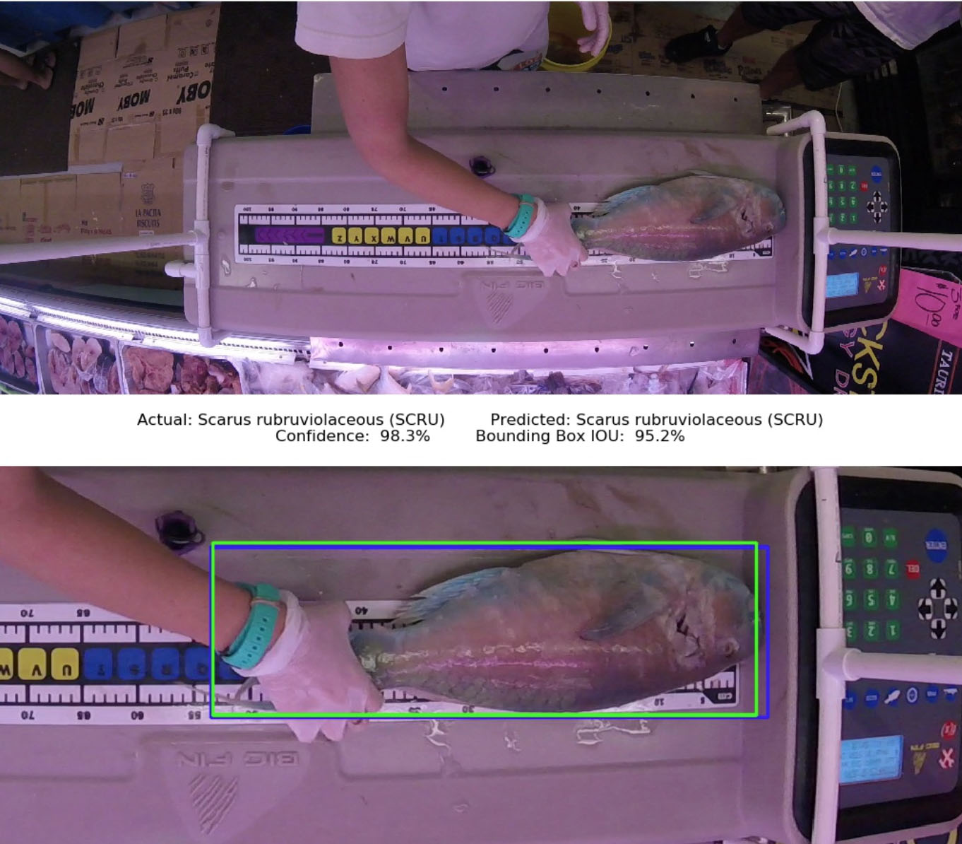
Figure: Image of a labeled fish with species and bounding box predictions.
We use the neural network architecture known as RetinaNet. RetinaNet was developed by Facebook AI Research in 2017 and was at that time the state-of-the-art in object detection. RetinaNet consists of three main components the ResNet backbone which is
used for to extract hierarchical features from the image the Feature Pyramid Network (FPN) which is used create multi-scale features the subnet components which map features into species and bounding box predictions
RetinaNet introduced the novel focal loss to help the network distinguish between the background and the objects[1]. In the context of fish detection, it is easy for a model to identify the background (i.e., the measuring board, the floor, and other parts
of the image that remain fixed throughout the video). On the other, the fish pose a more difficult problem--they appear less frequently and can appear in various locations in the image. At a high level, the focal loss gives more importance to
the fish predictions, thus encouraging the model to learn distinguishing information about the fish.
Results
Evaluation Metrics
Our model achieved an accuracy close to 99.9% using a small batch of training datasets. We split our data into a training and validation set and monitor progress on the validation set. We have a separate test set that contains 10% of the fish. We report
the test set performance here. The average accuracy is 94.2% and the average IOU is 85.7%. The accuracy describes how correctly the algorithm predicts the species, and IoU describes how closely the algorithm draw rectangular box around species
detected.
Table: Metrics for each species
Species
Accuracy
Intersection Over Union
No fish
89.01%
86.55%
Other
97.14%
85.93%
SCRU
96.94%
94.03%
MUFL
81.84%
80.13%
MUVA
97.93%
90.35%
LUKA
96.98%
79.72%
ACTR
95.08%
81.06%
ACOL
99.46%
88.18%
Table: Confusion matrix of predictions rows correspond to the predicted species, columns correspond to the ground truth species.
No fish
Other
SCRU
MUFL
MUVA
LUKA
ACTR
ACOL
No fish
9490
245
57
223
93
94
74
7
Other
425
8458
21
18
4
5
9
1
SCRU
181
0
2469
1
0
0
0
0
MUFL
99
0
0
1122
12
2
0
0
MUVA
162
0
0
0
5531
1
0
0
LUKA
126
0
0
7
8
3303
1
0
ACTR
21
0
0
0
0
1
1623
0
ACOL
158
4
0
0
0
0
0
1464
The confusion matrix shows the number of image frames that the algorithm predicted correctly and incorrectly. Columns correspond to the predicted species while rows correspond to the ground truth species and the corresponding values present the
number of predictions. The values in bold show correct predictions.
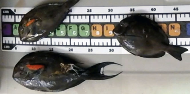
Using the annotated videos and RetinaNet, we were able to obtain on average 94.3% of accuracy on average with a minimum value of 90% and a maximum value of 99% (Table 2). Our IoU value was 85.7% on average ranging between 80% to 94%. While 70% IoU is
still enough for our application, the value was a bit lower than what we anticipated. The images below (Image 2) show differences of detection performance by different IoU values.
Video: Automatically Classifying Species in the Video
We learned that errors were introduced in the prediction due to annotation. The primary issue was an inconsistent start and end time for annotation of videos. Using different standards for start and end time by different annotators and videos of the annotation
caused many frames without fish. This reduced the annotation accuracy significantly. As reflected in the performance metrics (Table 3), one can see that frames with no fish were incorrectly predicting fish, thus lowering the accuracy. The first
row corresponds to frames when we predict too early (before the fish is aligned on the measuring board), and the first column corresponds to when we predict too late (as the fish is being removed from the measuring board).
We also learned that the algorithm does not recognize fish that are placed on a diagonal position and gives an IoU value equal to zero. It is primarily due to inconsistency of annotating fish of different positions. An example of this can be seen using
the link below to a video at the 11th second where the diagonally placed fish gets IoU close to zero. (https://drive.google.com/file/d/1Uo6oG61KSCyuyUfrrtLzx_ANMS7URdUO/view?usp=sharing)
If we slow down the video we can see that the model is actually making sensible predictions and the true source of error is due to inconsistencies in the way we have annotated the labels (the first and last frames with bounding boxes around the fish are
chosen subjectively by the annotator).
Discussion
We built the neural network with bio-sampling videos to reach the desired accuracy of classification for the 5 pre-selected species. Future potential applications of the machine learning algorithm with bio-sampling videos could include automated
annotation of the future bio-sampling videos, estimation of the number of fish during the video recording, or estimation of biological measurements.
While we were able to successfully achieve the desired accuracy of species identification with the preliminary report, with the full dataset of the annotated data, we observed more errors.
The main source of error comes from frames with no fish.
The errors in the first row of Table 3 occur when we predict there is a fish, but the ground truth states that there is no fish.
The errors in the first column of Table 3 occur when we predict there is no fish, but the ground truth states that there is a fish.
If we slow down the video we can see that the model is actually making sensible predictions and the true source of error is due to inconsistencies in the way we have annotated the labels (the first and last frames with bounding boxes around the fish are
chosen subjectively by the annotator). Thus, both these types of errors can be reduced if we standardize the labeling procedure.
As a rule of thumb in machine learning, more data leads to better results. Hence, we could improve our results by collecting and annotating more data. Furthermore, the images used to train the model come from bio sampling video. As a result, the current
model does not generalize well when presented with an image outside of this domain.
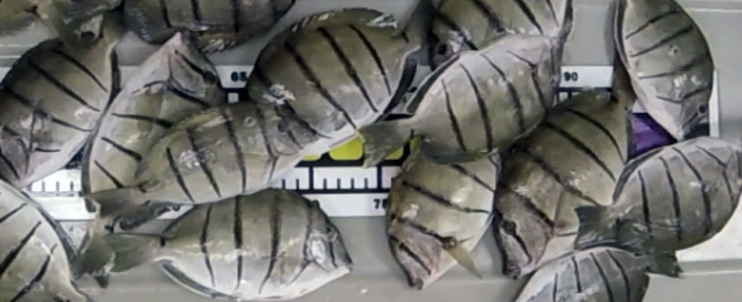
Figure 3: Acanthurus triostegus (ACTR)
The current model fails to detect the ACTR shown in Figure 3 because it is not from bio-sampling domain; it is not presented in the bio-sampling data collection environment. Similarly, if we want to make predictions for all the fish in an image,
we would need to annotate all the fish in an image. This would require more annotation work, but the current model architecture and training procedure could be used.
We used data augmentation during training to make the model more robust. We can also use data augmentation at inference time (making predictions, after training) to increase accuracy at the expense of increasing computation time, this is known as test-time
augmentation (TTA) (A. Krizhevsky, 2012).
In this pilot project, we used the RetinaNet architecture which was the state-of-the-art in 2017. However, deep learning is very fast-moving field and there are currently better (faster and more accurate) architectures. It is not hard to swap out RetinaNet
for a more modern architecture.
We suggest the following modern architectures:
If speed is important, then use YOLO3 (J. Redmon et al, 2018). RetinaNet’s requires about 0.5s to make a prediction for each frame. We can expect a 3-5x speed up with YOLO3.
If better accuracy is important, then use Mask-RCNN (K. He et al., 2017). Mask-RCNN performs about 30% better than RetinaNet on the COCO dataset ( Lin TY. et al., 2014). We can expect a similar improvement with our data.